D&D.Sci, problem 2
This post is part of my "dnd.sci" series.
This is the first part I'm doing with a "proper" toolchain. Relearning Jupyter, Pandas, and Matplotlib at once is going to be difficult enough without throwing machine-learning algorithms into the mix. Consequently, I'm going to import linear regression and r-square from scikit-learn, but that's it.
I'm making the spreadsheet for the last problem, plus the data and notebooks for this one, available through my GitHub account.
Problem statement
You are hired to obtain magic items for a sorcerer. You have 200 gold pieces (gp) and access to the local magic shop. The sorcerer demands that the items, when sacificed for their power, yield enough mana to complete his spell. You don't know how much mana is contained on each item, but you have access to the sorcerer's meticulous records. If the mana supplied is insufficient you will owe the sorcerer his 200gp back, otherwise you can keep what you don't spend.
Data cleanup
We have two sources of data: the sacrifice data provided by Wakalix the Wizard, and the store list collected by us. I did some cleaning, reshaping, and renaming, and then saved everything to a new file.
Sacrifice
There are four columns to the sacrifice data: "Item name", "Glow color", "Thaumometer reading", and "Mana gained from sacrifice".
The item names seem to conform to the format "Item of Enchantment +d" (eg: "Warhammer of Rage +1"). There are some items that don't seem to have any modifier.
We can check if we have accounted for everything by using a regular expression.
data["Item name"].str.match("\w+ of \w+( \+\d)?").all()
A regular expression is a string that describes a different string. In the above "\w+" means some (at least one) word-character (letters, numbers, dashes, and underscores, I believe). Because "+" is used to indicate repetition, when we talk about actual plus signs we need to escape them; so "( +\d)?" stands for "optionally, a space, a plus sign, and a digit".
All of the items follow the pattern, so we can split the name into its components. The modifiers range from 1 to 8, so I took all of the missing modifiers and treated them as "+0".
The names of the columns are pretty verbose, and we'll be typing them a bunch, so I set them to "item", "enchant", "mod", "color", "thmm", and "mana".
Store
The item names in the store data follow the same pattern (I checked by hand this time around, they are very few). I split and cleaned them with the same code.
The color field had the colors capitalized, so I had to lowercase them to match the sacrifice data.
Obviously there was no mana field, since guessing that is the whole point of the exercise.
Analysis
No matter how much analysis we do, we cannot know how much mana each item will give. There is a real risk of overthinking things when doing these analyses. We want to make a profit from the transaction; instead of analyzing forever, we should pay attention to whether we have enough information to do that. I'm going to be doing a best effort guess as soon as possible, and refine it as we go along.
There is also the issue of "what even is success?".
- We like money, and want more of it
- We don't care for how much mana Wakalix gets, and neither does he. We only care if we meet the threshold.
- Failing to get enough mana has a limited downside (we owe 200gp).
- I don't know how much 200gp is, but I'm going to assume we are not particularly risk-averse.
From these points, I propose we define our performance as the expected value of the deal. \(E(deal) = U \times P(mana >= 120) - D \times P(mana < 120)\). Where U is the size of the upside, and D is the size of the downside.
I'm assuming that Wakalix just wants his money back, instead of asking for compensation on top of the money lost, so D is not 200gp, but whatever money we actually spent. If we call \(\varepsilon\) our expenditures, we can say \(E(deal) = (200gp - \varepsilon) \times P(mana >= 120) - \varepsilon \times P(mana < 120)\).
Guess 1
Let's start with the obvious: mean item mana is 20.5. If we assume that price and mana are uncorrelated, picking the six cheapest items yields 123 expected mana for 194 gp, which is just under budget.
I did not calculate the probability of ruin (I'm lazy) but it can be done by repeatedly picking six random items from Wakalix's list, and checking whether they add up to 120 mana or not.
Guess 2
Let's bring in the Thaumometer into account. A linear regression from thmm to mana yields an intercept of 13.6, slope of 0.25, and r-squared of 0.10. A couple of things are obvious from that:
- the r-squared is terrible, so the thaumometer tells us pretty much nothing
- this is reinforced by the slope of 0.25; mana is not sensitive to such an uninformative predictor
Picking the six items with the best mana/gp yields 141 expected mana for 197 gp. Again, I didn't calculate the expected value of the deal, but with 21 points of mana cushion, I'd say we'd pass. However, we would make no money.
Intermission
Let's take a closer look at the thmm-mana response. A thaumometer-mana scatterplot would have a lot of repeated or tightly-clustered readings, distorting our perception of hot spots. We'll use a a hexbin plot. Hexbin plots split the plane into areas and show us how many readings fell on each area. It's like histograms, but for 2D data.
Why hexagons? I found a paper about it1, but even after reading it I don't have much of a reason.
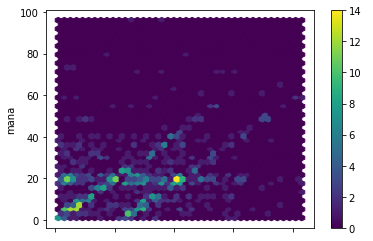
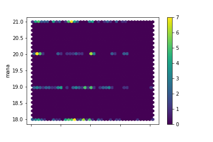
Ok, that is interesting:
- There are two parallel diagonals, one from (0,0), one shifted right.
- There is a horizontal line at about 20 mana.
This suggest the following:
- Some items are being correctly predicted, with maybe a slope adjustment needed.
- Some items are basically correctly predicted, but are overestimated by some constant amount.
- Some items are predictably 20 mana, but the thaumometer is not picking it up at all. The line is horizontal because the correct value, 20, is associated to all sorts of different readings, resulting in a big horizontal spread. If the items were correctly predicted, they would show up as a bright spot at (20, 20).
Turns out that drawing a separate hexbin plot per color is pretty easy:
data.groupby("color").plot.hexbin(x="thmm", y="mana", gridsize=40, cmap="viridis")
x and y are what you'd expect, gridsize tells us how many hexagons per side there are (in this case, there are 40x40=1600 bins), and cmap defines a color map, ie a mapping from numbers to a palette of colors. "viridis" is the name of a palette that comes built-in with Matplotlib, which Pandas uses to do the graphs.
blue
green
red
yellow
Wonderful, I could not have hoped for cleaner data:
- The Thaumometer predicts mana only for blue items. This is why the relation was so weak in general. If we limit the regression to blue item data we'll get some really precise predictions. We still have the double-line to explain, though.
- Yellow items all fall in the 18-21 mana range.
Guess 3
Let's incorporate all we know so far into a prediction function:
def predictor(color, thmm):
    if color == "yellow":
        return 19.5
    elif color == "blue":
        return linear_regressor.predict(np.array([thmm], ndmin=2))[0][0]
    else:
        return 22.9
19.5 is the mean of the yellow items (eyeballed). 22.9 is the mean of the greens and reds. The linear regressor returns an r-squared of 0.28 (much better, and better than anything I could do for problem 1), slope of 0.66, intercept of 0.02.
Picking the four items with the best mana/gp yields 119.9 expected mana, for 139 gp. Not bad! But I smell weakness. We can figure out where that double-line comes from.
Guess 4
Let's calculate the error for each blue item and see if items, enchants, or modifiers tell us anything:
blues = data[data["color"] == "blue"]
blues.eval('error = thmm - mana').groupby("item")["error"].mean()
item
Amulet       22.000000
Axe           0.538462
Battleaxe     0.357143
Hammer        0.400000
Longsword     0.363636
Pendant      21.975610
Plough        0.375000
Ring         22.121951
Saw          -0.058824
Sword         0.000000
Warhammer     0.000000
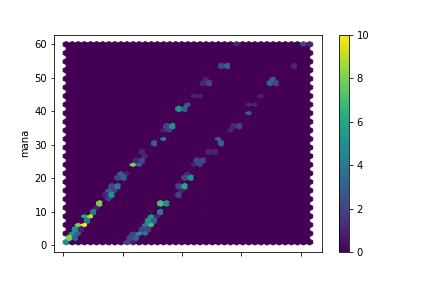
First try! Almost no error anywhere, but consistent errors in three categories: Amulets, Pendants, and Rings. The Thaumometer has a thing for jewelry! Let's adjust for that and see if there is any residue.
blues.eval('adj_thmm = thmm - 22*(item in ["Amulet", "Pendant", "Ring"])', inplace=True)
blues.plot.hexbin(x="adj_thmm", y="mana", gridsize=40, cmap="viridis")
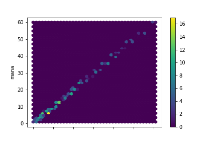
Beautiful. r-squared of 0.996. Maximum absolute error of 1 mana.
def predictor(item, color, thmm):
    if color == "yellow":
        return 19.5
    elif color == "blue":
        if item in ["Amulet", "Pendant", "Ring"]:
            return thmm - 22
        else:
            return thmm
    else:
        return data.query('color == @color')["mana"].mean()
Applying the predictor to the entire dataset, we obtain an r-squared of 0.42.
Picking the four items with the best mana/gp yields an expected 136.5 mana for 142 gp.
At this point we can stop with a nice guaranteed income. Picking among blues and yellows only (remember, we got these down to 1 or 2 mana points of error) we get 129 mana for 145 gp. But I was curious to see if we could squeeze out anything more, so I decided to take a little look at the reds and greens, which so far had eluded me.
Guess 5
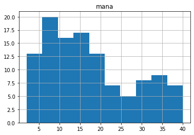
I plotted histograms for every red item, broken by item type.
reds.hist(column="mana", by="item", figsize=(13,8), sharex=True, sharey=True, bins=20)
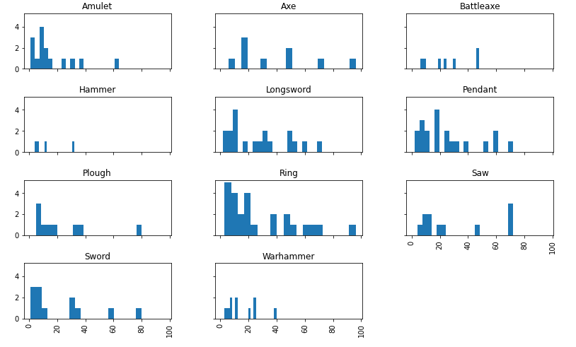
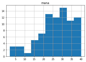
Since that didn't look like anything to me, I did the same for enchantment, then by modifier. Then I repeated everything with the green items.
At last, when I was about to give up, I spotted a pattern:
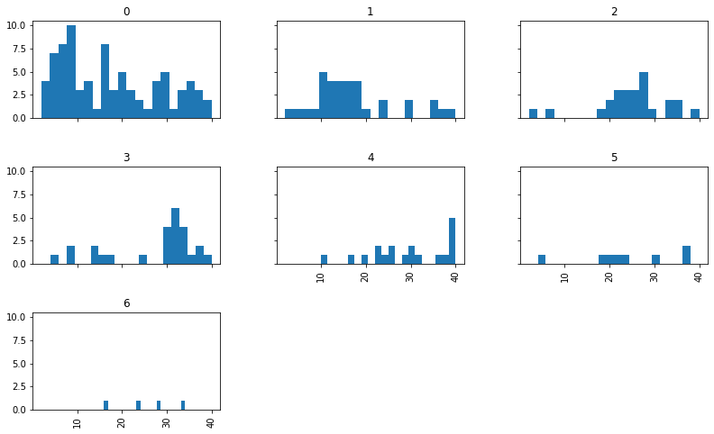
The items seem to shift right as we go from +0 modifier, to +1, to +2, etc. Looking at the means, there is a noticeable jump from +1 to +2.
mod
0    17.432099
1    17.294118
2    25.280000
3    27.153846
4    29.473684
5    24.250000
6    25.500000
If we split the green items into low-modifier (+0/+1) and high-modifier groups, we can see the jump.
green, lo-mod
green, hi-mod
I didn't originally notice a modifier-mana relation in the red items, but now I have a reason to look again:
reds.eval('himod = mod >= 2').hist(column="mana", by="himod", sharex=True, sharey=True, figsize=(13,8))
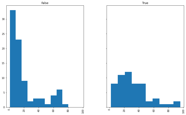
red items: lo-mod (left) and hi-mod (right)
We can now construct and run our final predictor:
def predictor(item, mod, color, thmm):
    if color == "yellow":
        return 19.5
    elif color == "blue":
        if item in ["Amulet", "Pendant", "Ring"]:
            return thmm - 22
        else:
            return thmm
    elif color == "red":
        if mod < 2:
            return 20.5
        else:
            return 32.3
    else: # color is green
        if mod < 2:
            return 17.4
        else:
            return 26.8
r-squared of 0.47. A modest but welcome improvement. How does this affect our available options?
Picking the four items with the best mana/gp yields 143 mana for 143 gp. The numbers aren't much different, but the additional information has changed our item selection. Now we have two blue item and two greens. The blues account for \(90 \pm 2\) mana. To make it to 120, we need another 30 mana from two green items (modifiers +2 and +4).
What are the odds? Well, we can do what I should have done at the begining: random resampling. Why resampling? In short: because we don't want to get tripped up by how the population is distributed.
We know that, among high-modifier green items, the mean item yields 26.8 mana when sacrificed. If all items yielded exactly that, we'd have no variation, and therefore no risk. If one in ten items yielded 268 mana while the others yielded 0, we would have a 19% chance of having way too much mana, and a 81% chance of nothing, but we'd still see the same 26.8 mean mana figure.
When you have a lot of items, each one independently contributing a small percentage of the expected total, the Central Limit Theorem tells you the sum is going to be normal (bell-shaped), even if the individual contributions are not normal. It even tells you the correct standard deviation. We have two items. There is some debate over how many is "a lot", but in this case we can confidently say we don't have "a lot" of items. So we can't rely on the Central Limit Theorem to calculate our chances.
Resampling has limits, mind you. There is nothing stopping you from resampling ten thousand times and coming up with a very confident estimate of your odds… from six samples. We have 82 items in the "green, high-modifier" category. That yields 82*82 = 6724 pairs (if we allow sampling the same item more than once). Sampling about 1000 pairs seems about right.
Laplace's Law of Succession tells us to pretend we have seen an extra hit and miss when calculating our totals. To make the denominator a nice round number, I'll use 998 samples.
pop = data.query('color == "green" and mod >= 2')["mana"]
samp = pd.Series([ pop.sample(2, replace=True).sum() for i in range(0,998) ])
samp.apply(lambda x: x >= 30).value_counts()
True     965
False     33
966/1000 is 96.6% chance of success. Not bad, but restricting our choice to blues and yellows bumps that up to 100% (as long as I haven't fucked up the model). Is the extra gold we'd pocket worth the extra risk?
- expected value of safe option: 55 gp
- expected value of greedy option: 51 gp
- success: 96.6% x 57gp = 55.1
- fail: 3.4% x -143gp = -4.9
No, it isn't. Our final lineup of items: Pendant of Hope, Hammer of Capability, Plough of Plenty, Warhammer of Justice +1. Expected mana: 129 (124-134). Cost: 145gp.
-
Lewin-Koh, Nicholas. “Hexagon Binning: An Overview,” January 8, 2021. https://cran.r-project.org/web/packages/hexbin/vignettes/hexagon_binning.pdf. ↩